Chainerのチュートリアルを試してみた(畳み込みを深くする編)
Chainerのチュートリアルを試してみました。層をブロックにして、深いネットワークを作ってみます。
目次
チュートリアルの内容
Chainerのチュートリアルは本家でも公開されてますが、今回試してみたのは こちらのサイトのもの です。リンク先のサイトではJupyter notebookを使う前提で書かれているのですが、本投稿ではローカル環境でのPythonで実行します。
実行した環境は、Windows10 64bit、Python 3.7、Chainer 6.1、CUDA 10.1です。
CIFAR10の画像の分類をします。
データセットの準備
Chainerの便利機能でダウンロードして分割したCIFAR10のデータセットを使用します。ダウンロードの方法は 以前の投稿 の「データセットのダウンロード」の箇所を参照してください。
深いネットワークを作る
畳み込み層と前後する一連の層や、全結合層と前後する一連の層を塊(ブロック)にして、そのブロックをつなげることで深い(長い)ネットワークを作ります。今回作るネットワーク全体はこんな感じです。
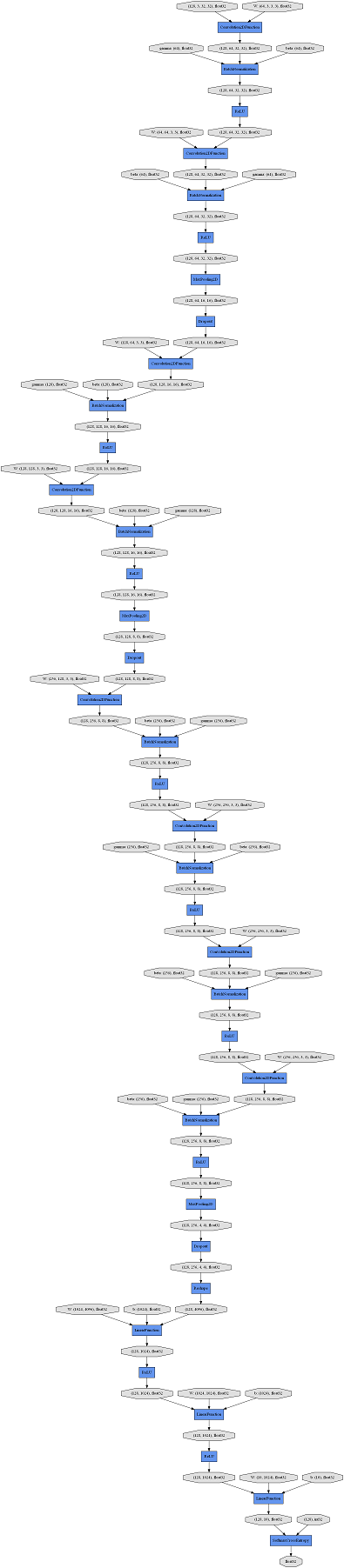
ConvBlockというクラスは、畳み込み層のブロックを定義するクラスです。入力に対して、畳み込み、バッチ正規化、ReLU(、マックスプーリング、ドロップアウト)をひとまとめにしています。
LinearBlockというクラスは、全結合層のブロックを定義するクラスです。入力に対して、全結合、ReLU(、ドロップアウト)をひとまとめにしています。
このブロックの中にifで分岐を書けるのですね。
これらのブロックをDeepCNNというChainListを継承したクラスに列挙することで、深いネットワークを作ります。
import pickle
import numpy
import random

import chainer
import chainer.cuda
import cupy
import chainer.links as L
import chainer.functions as F
from chainer import iterators
from chainer import optimizers
from chainer import training
from chainer.training import extensions
from chainer import serializers

# 畳み込み層部分の定義をするクラス
class ConvBlock(chainer.Chain):

    def __init__(self, n_ch, pool_drop=False):
        w = chainer.initializers.HeNormal()
        super(ConvBlock, self).__init__()
        with self.init_scope():
            self.conv = L.Convolution2D(None, n_ch, 3, 1, 1, nobias=True, initialW=w) # 畳み込み層
            self.bn = L.BatchNormalization(n_ch) # バッチノーマリゼーション層
        self.pool_drop = pool_drop

    def __call__(self, x):
        h = F.relu(self.bn(self.conv(x))) # 入力を畳み込んで、バッチ正規化して、ReLUを通す
        if self.pool_drop: # pool_dorpがTrueのときは、マックスプーリングして、ドロップアウトする
            h = F.max_pooling_2d(h, 2, 2)
            h = F.dropout(h, ratio=0.25)
        return h

# 全結合層部分の定義をするクラス
class LinearBlock(chainer.Chain):

    def __init__(self, drop=False):
        w = chainer.initializers.HeNormal()
        super(LinearBlock, self).__init__()
        with self.init_scope():
            self.fc = L.Linear(None, 1024, initialW=w) # 全結合層
        self.drop = drop

    def __call__(self, x):
        h = F.relu(self.fc(x)) # 入力を全結合して、ReLuを通す
        if self.drop: # dropがTrueのときは、ドロップアウトする
            h = F.dropout(h)
        return h

# ネットワーク全体の定義をするクラス
class DeepCNN(chainer.ChainList):

    def __init__(self, n_output):
        super(DeepCNN, self).__init__(
            ConvBlock(64),
            ConvBlock(64, True),
            ConvBlock(128),
            ConvBlock(128, True),
            ConvBlock(256),
            ConvBlock(256),
            ConvBlock(256),
            ConvBlock(256, True),
            LinearBlock(),
            LinearBlock(),
            L.Linear(None, n_output)
        )

    def __call__(self, x):
        for f in self:
            x = f(x)
        return x

# 学習を実行する関数
def train(network_object, batchsize=128, gpu_id=0, max_epoch=20, train_dataset=None, valid_dataset=None, test_dataset=None, postfix='', base_lr=0.01, lr_decay=None):

    # 1. データセットの読み込み
    with open('test.pickle', mode='rb') as fi1:
        test = pickle.load(fi1)
    with open('train.pickle', mode='rb') as fi2:
        train = pickle.load(fi2)
    with open('valid.pickle', mode='rb') as fi3:
        valid = pickle.load(fi3)

    # 2. イテレーターの作成(データセットをバッチで取り出せるようにする)
    train_iter = iterators.SerialIterator(train, batchsize)
    valid_iter = iterators.SerialIterator(valid, batchsize, False, False)

    # 3. ネットワークのインスタンスを作る
    net = L.Classifier(network_object)

    # 4. オプティマイザーの作成(学習量の計算の設定)
    optimizer = optimizers.MomentumSGD(lr=base_lr).setup(net)
    optimizer.add_hook(chainer.optimizer.WeightDecay(0.0005))

    # 5. アップデーターの作成(ネットワークのパラメーターのアップデート)
    updater = training.StandardUpdater(train_iter, optimizer, device=gpu_id)

    # 6. トレーナーの作成(学習サイクルの実行)
    trainer = training.Trainer(updater, (max_epoch, 'epoch'), out='{}_cifar10_{}result'.format(network_object.__class__.__name__, postfix))

    # 7. トレーナーのオプションの設定
    trainer.extend(extensions.LogReport())
    trainer.extend(extensions.observe_lr())
    trainer.extend(extensions.Evaluator(valid_iter, net, device=gpu_id), name='val')
    trainer.extend(extensions.PrintReport(['epoch', 'main/loss', 'main/accuracy', 'val/main/loss', 'val/main/accuracy', 'elapsed_time', 'lr']))
    trainer.extend(extensions.PlotReport(['main/loss', 'val/main/loss'], x_key='epoch', file_name='loss.png'))
    trainer.extend(extensions.PlotReport(['main/accuracy', 'val/main/accuracy'], x_key='epoch', file_name='accuracy.png'))
    trainer.extend(extensions.dump_graph('main/loss'))
    if lr_decay is not None:
        trainer.extend(extensions.ExponentialShift('lr', 0.1), trigger=lr_decay)
    trainer.run()
    del trainer

    # 8. 評価
    test_iter = iterators.SerialIterator (test, batchsize, False, False)
    test_evaluator = extensions.Evaluator(test_iter, net, device=gpu_id)
    results = test_evaluator()
    print('Test accuracy:', results['main/accuracy'])

    return net

# 乱数を初期化する関数
def reset_seed(seed=0):
    random.seed(seed)
    numpy.random.seed(seed)
    if chainer.cuda.available:
        chainer.cuda.cupy.random.seed(seed)

# cuDNNのautotuneを有効にする
chainer.cuda.set_max_workspace_size(512 * 1024 * 1024)
chainer.config.autotune = True

# 乱数の初期化
reset_seed(0)

# 学習の実行
net = train(DeepCNN(10), max_epoch=100, base_lr=0.1, lr_decay=(30, 'epoch'))

# 学習結果の保存
serializers.save_npz('my_cifar10.model', net)
今回はGPUで計算しますので、autotuneを有効にしてみました。
Visual Studio Codeのpylintがchainer.cudaのメンバーが無いという警告を出してきたのでちょっと焦りましたが、問題なくGPUで計算してくれたようです。
epoch       main/loss   main/accuracy  val/main/loss  val/main/accuracy  elapsed_time  lr
1           2.6437      0.144531       2.2232         0.16582            20.6501       0.1
2           2.12134     0.207919       2.00311        0.267578           39.8627       0.1
3           1.88175     0.28835        1.96174        0.292969           58.8182       0.1
4           1.73099     0.345503       1.77057        0.312891           77.8201       0.1
5           1.57302     0.417713       1.6491         0.391016           96.6805       0.1
6           1.37428     0.496316       1.44605        0.480273           115.618       0.1
7           1.20373     0.565104       1.195          0.567578           134.556       0.1
8           1.09236     0.609397       1.2061         0.573438           153.542       0.1
9           0.983244    0.65261        1.04837        0.649805           172.479       0.1
10          0.910236    0.679532       0.890074       0.689648           191.431       0.1
11          0.839646    0.710005       1.12711        0.637891           210.407       0.1
12          0.777537    0.73275        1.24749        0.60293            229.283       0.1
13          0.750183    0.742188       0.823973       0.72168            248.311       0.1
14          0.702904    0.76035        0.71562        0.75332            267.239       0.1
15          0.674656    0.769664       0.906134       0.70332            286.208       0.1
16          0.659935    0.779336       0.753152       0.737109           305.08        0.1
17          0.617898    0.791926       0.633969       0.785547           324.063       0.1
18          0.603082    0.798074       0.989168       0.675977           343.001       0.1
19          0.587477    0.803641       0.802272       0.747656           361.917       0.1
20          0.569411    0.809104       0.843102       0.726953           380.843       0.1
21          0.557242    0.811944       0.705192       0.762891           399.715       0.1
22          0.538812    0.822088       1.57609        0.574023           418.659       0.1
23          0.527007    0.821937       0.711417       0.783594           437.541       0.1
24          0.527024    0.82342        1.01725        0.662109           456.515       0.1
25          0.504342    0.829967       0.98378        0.703125           475.428       0.1
26          0.499243    0.833178       0.943754       0.702539           494.347       0.1
27          0.498686    0.833341       2.72165        0.434961           513.275       0.1
28          0.477141    0.840589       0.789254       0.74375            532.147       0.1
29          0.471671    0.841819       0.669663       0.788477           551.122       0.1
30          0.476996    0.84148        0.586559       0.80293            570.04        0.1
31          0.300428    0.897905       0.39851        0.877148           588.969       0.01
32          0.221266    0.92488        0.36525        0.881641           607.863       0.01
33          0.191751    0.933993       0.357381       0.89043            626.788       0.01
34          0.170519    0.941628       0.347432       0.892969           645.745       0.01
35          0.153229    0.946136       0.357087       0.886328           664.709       0.01
36          0.140532    0.951127       0.354779       0.889648           683.689       0.01
37          0.13109     0.95426        0.361992       0.891016           702.585       0.01
38          0.118159    0.958629       0.392906       0.887695           721.536       0.01
39          0.109702    0.962362       0.387895       0.889258           740.475       0.01
40          0.102641    0.964134       0.405599       0.888281           759.706       0.01
41          0.0972486   0.966397       0.394764       0.892773           778.749       0.01
42          0.0915414   0.967993       0.402179       0.892773           797.765       0.01
43          0.0863423   0.970104       0.412282       0.888477           816.733       0.01
44          0.0878853   0.969306       0.432859       0.882422           835.611       0.01
45          0.078483    0.972168       0.432829       0.883984           854.549       0.01
46          0.0750526   0.97447        0.412971       0.892187           873.462       0.01
47          0.0684961   0.976318       0.420595       0.890039           892.409       0.01
48          0.0686924   0.976451       0.478586       0.880273           911.282       0.01
49          0.070054    0.975852       0.444838       0.883008           930.2         0.01
50          0.0713485   0.975053       0.433133       0.884961           949.11        0.01
51          0.0656244   0.977364       0.465228       0.885156           967.978       0.01
52          0.0604113   0.979115       0.467371       0.878516           986.931       0.01
53          0.0677948   0.976496       0.467753       0.880078           1005.82       0.01
54          0.0590325   0.979359       0.491907       0.88125            1024.74       0.01
55          0.0612465   0.978966       0.451046       0.886914           1043.63       0.01
56          0.0653968   0.977472       0.49247        0.879297           1062.62       0.01
57          0.060906    0.979137       0.481422       0.882422           1081.63       0.01
58          0.06187     0.979167       0.467294       0.886523           1100.55       0.01
59          0.0618526   0.978826       0.468995       0.88457            1119.48       0.01
60          0.0565759   0.980257       0.567624       0.86543            1138.38       0.01
61          0.0374251   0.98746        0.415678       0.892773           1157.38       0.001
62          0.0229866   0.993122       0.419805       0.891602           1176.31       0.001
63          0.0192019   0.994074       0.419598       0.894336           1195.31       0.001
64          0.0174565   0.994925       0.422318       0.897656           1214.2        0.001
65          0.0162033   0.994851       0.427115       0.897656           1233.15       0.001
66          0.0150596   0.995472       0.429711       0.896484           1252.13       0.001
67          0.012677    0.996439       0.432503       0.895703           1271.12       0.001
68          0.0118089   0.99656        0.437222       0.898828           1290.15       0.001
69          0.0129675   0.996216       0.444267       0.896094           1309.03       0.001
70          0.0108742   0.996893       0.444565       0.900195           1327.97       0.001
71          0.01087     0.996995       0.447843       0.89707            1346.84       0.001
72          0.00934628  0.997314       0.450479       0.898242           1365.84       0.001
73          0.00934687  0.997181       0.459053       0.898633           1384.83       0.001
74          0.00939448  0.997106       0.460052       0.899219           1403.78       0.001
75          0.00902866  0.997514       0.455976       0.899023           1422.77       0.001
76          0.00872597  0.997507       0.465737       0.898633           1442          0.001
77          0.0093198   0.997026       0.46898        0.898633           1461.14       0.001
78          0.00859233  0.997396       0.460254       0.898047           1480.13       0.001
79          0.00779859  0.997803       0.463143       0.899805           1499.1        0.001
80          0.00736309  0.997975       0.459977       0.899805           1518.02       0.001
81          0.0081748   0.99747        0.464284       0.897461           1537.02       0.001
82          0.00776547  0.997714       0.462811       0.898438           1556.03       0.001
83          0.00709248  0.998108       0.466836       0.9                1575.1        0.001
84          0.00721658  0.99818        0.467964       0.898828           1594.38       0.001
85          0.00739202  0.997997       0.467479       0.899609           1613.31       0.001
86          0.00681072  0.998202       0.458913       0.900195           1632.22       0.001
87          0.00629826  0.998353       0.46128        0.899609           1651.1        0.001
88          0.00676739  0.997958       0.467949       0.9                1670.01       0.001
89          0.00704037  0.998291       0.472412       0.902148           1688.89       0.001
90          0.00633939  0.998197       0.466698       0.899219           1707.76       0.001
91          0.00567754  0.998691       0.462024       0.9                1726.76       0.0001
92          0.00576062  0.998642       0.461816       0.898242           1745.61       0.0001
93          0.00595025  0.998668       0.462708       0.899219           1764.62       0.0001
94          0.00589382  0.998353       0.463547       0.9                1783.62       0.0001
95          0.00611592  0.998335       0.459985       0.900781           1802.67       0.0001
96          0.00645041  0.998064       0.461833       0.9                1821.66       0.0001
97          0.00565064  0.998491       0.460635       0.900586           1840.71       0.0001
98          0.00585507  0.998491       0.459271       0.899414           1859.62       0.0001
99          0.00535949  0.998665       0.468896       0.9                1878.5        0.0001
100         0.00535571  0.998668       0.466266       0.901172           1897.59       0.0001
Test accuracy: 0.89685524
精度がおよそ90%になりました。
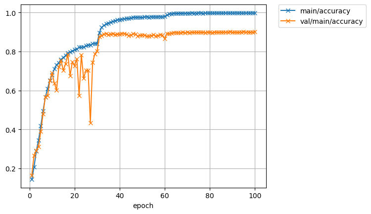
30エポックのあたり(学習率Ir)を小さくしたところでガンッと精度が上がってます。
推論してみた
では学習したモデルを使って、テストデータの推定をしてみます。
今回は、100枚のテスト画像に対して、教師データと推定値が異なるものだけを表示するようにしてみました。
import pickle
import matplotlib.pyplot as plt

import chainer
import chainer.links as L
import chainer.functions as F
from chainer import serializers

# 畳み込み層部分の定義をするクラス
class ConvBlock(chainer.Chain):

    def __init__(self, n_ch, pool_drop=False):
        w = chainer.initializers.HeNormal()
        super(ConvBlock, self).__init__()
        with self.init_scope():
            self.conv = L.Convolution2D(None, n_ch, 3, 1, 1, nobias=True, initialW=w) # 畳み込み層
            self.bn = L.BatchNormalization(n_ch) # バッチノーマリゼーション層
        self.pool_drop = pool_drop

    def __call__(self, x):
        h = F.relu(self.bn(self.conv(x))) # 入力を畳み込んで、バッチ正規化して、ReLUを通す
        if self.pool_drop: # pool_dorpがTrueのときは、マックスプーリングして、ドロップアウトする
            h = F.max_pooling_2d(h, 2, 2)
            h = F.dropout(h, ratio=0.25)
        return h

# 全結合層部分の定義をするクラス
class LinearBlock(chainer.Chain):

    def __init__(self, drop=False):
        w = chainer.initializers.HeNormal()
        super(LinearBlock, self).__init__()
        with self.init_scope():
            self.fc = L.Linear(None, 1024, initialW=w) # 全結合層
        self.drop = drop

    def __call__(self, x):
        h = F.relu(self.fc(x)) # 入力を全結合して、ReLuを通す
        if self.drop: # dropがTrueのときは、ドロップアウトする
            h = F.dropout(h)
        return h

# ネットワーク全体の定義をするクラス
class DeepCNN(chainer.ChainList):

    def __init__(self, n_output):
        super(DeepCNN, self).__init__(
            ConvBlock(64),
            ConvBlock(64, True),
            ConvBlock(128),
            ConvBlock(128, True),
            ConvBlock(256),
            ConvBlock(256),
            ConvBlock(256),
            ConvBlock(256, True),
            LinearBlock(),
            LinearBlock(),
            L.Linear(None, n_output)
        )

    def __call__(self, x):
        for f in self:
            x = f(x)
        return x

# 推論を実行する関数
def predict(net, image_id):
    x, t = test[image_id]
    with chainer.using_config('train', False), chainer.using_config('enable_backprop', False):
        y = net.predictor(x[None, ...]).data.argmax(axis=1)[0]

    if t != y:
        plt.imshow(x.transpose(1, 2, 0))
        plt.text(1,1, cls_names[t], color='red')
        plt.text(1,2, cls_names[y], color='red')
        plt.show()

# テストデータのラベル
cls_names = ['airplane', 'automobile', 'bird', 'cat', 'deer', 'dog', 'frog', 'horse', 'ship', 'truck']

# テストデータの読み込み
with open('test.pickle', mode='rb') as fi1:
    test = pickle.load(fi1)

# ネットワークのインスタンスの作成
infer_net = L.Classifier(DeepCNN(10))

# ネットワークの学習済みパラメーターの読み込み
serializers.load_npz('my_cifar10.model', infer_net)

# 推論の実行
for i in range(10, 110):
    predict(infer_net, i)
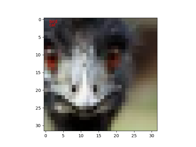
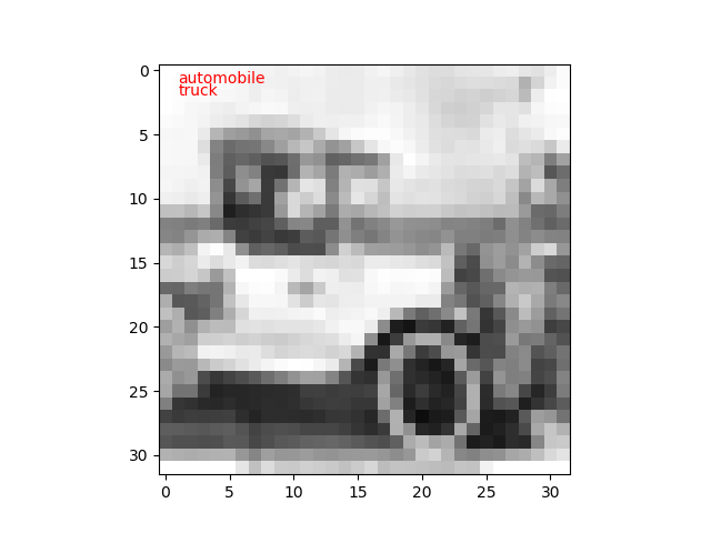
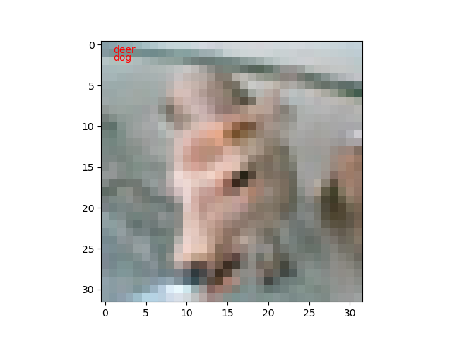
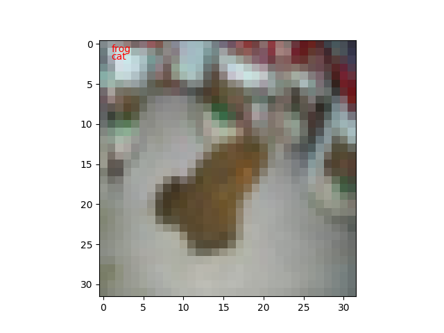
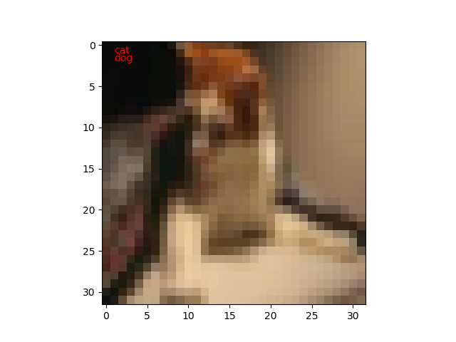
私も間違えそうな画像があります。
公開日
広告
Chainerカテゴリの投稿
- ChainerCVで使える画像のデータ拡張
- ChainerCVで画像を出力する方法
- ChainerCVのResNetを使う
- ChainerCVのSSDに学習させてみた
- ChainerCVのデモンストレーションプログラムを読んでみた
- ChainerCVのデモンストレーションプログラムを読んでみた(推論編)
- Chainerが出力するネットワーク構造図をGraphvizで見る
- Chainerで数字を分類してみた
- ChainerのSSDのデモで物体検出をしてみる
- Chainerのチュートリアルを試してみた
- Chainerのチュートリアルを試してみた(ChainerCVでデータ拡張編)
- Chainerのチュートリアルを試してみた(データ拡張編)
- Chainerのチュートリアルを試してみた(トレーナー編)
- Chainerのチュートリアルを試してみた(畳み込みを深くする編)
- Chainerのチュートリアルを試してみた(畳み込み編)
- Chainerのデータセットの作り方(ラベル付き画像編)
- VoTTのPascal VOC出力をChainerCVのデータセットとして読み込んでみた