Chainerのチュートリアルを試してみた(トレーナー編)
Chainerのチュートリアルを試してみました。トレーナーを使ったものです。
目次
Chainerとは
Chainer とは、言わずと知れたPython用のディープラーニングフレームワークです。
本家でチュートリアルを公開されてますが、今回試してみたのは こちらのサイトのもの で、中盤に書かれているtrainerを使用した場合です。
試した環境は、Windows10 64bit、Python 3.7、Chainer 6.1です。GPUは使用しません。 参考にしたサイトはJupyter notebookでの実行を前提に書かれていますが、この投稿ではVisual Studio Codeで実行しました。
内容としては、簡単なネットワークを使ってMNISTの画像セットの分類をするというものです。
基本的にはチュートリアルにあるコードを、ローカルで動かせるように改変しながらトレースしたものです。
UpdaterとTrainer
コードの途中でL.Classifierというメソッドが出てきますが、これはネットワークのインスタンスにロスを計算する機能を追加するものです。
UpdaterはIteratorとOptimizerを使って、ミニバッチを作り、順方向の計算をして、ロスを計算して、パラメーターのアップデートをしてくれます。
Updaterが一連の学習の手順を実行してくれるのですが、そのUpdaterを使って学習全体を管理するのがTrainerです。学習する回数や、ログの出力などの制御をします。
データの準備
トライアンドエラーで何度も実行することを想定しまして、Chainerの便利機能でダウンロードしたMNISTデータをローカルに保存して利用します。手順は 前の投稿 を参照してください。
学習
おおまかに言って、こんな流れです。
データセットの準備をする。
イテレーターを作る。
ネットワークを作る。
オプティマイザーを作ってネットワークを渡す。
アップデーターにイテレーターとオプティマイザーを渡す。
トレーナーにアップデーターを渡して学習を実行する。
学習結果を保存する。
コードがかなりすっきりするように感じますね。
import pickle
import matplotlib.pyplot as plt
import random
import numpy

import chainer
from chainer.datasets import split_dataset_random
from chainer import iterators
import chainer.links as L
import chainer.functions as F
from chainer import optimizers
from chainer import training
from chainer.training import extensions

# 乱数を初期化する関数
def reset_seed(seed=0):
    random.seed(seed)
    numpy.random.seed(seed)
    if chainer.cuda.available:
        chainer.cuda.cupy.random.seed(seed)

# ネットワークを定義するクラス
class MLP(chainer.Chain):

    def __init__(self, n_mid_units=100, n_out=10):
        super(MLP, self).__init__()

        # パラメータを持つ層
        with self.init_scope():
            self.l1 = L.Linear(None, n_mid_units)
            self.l2 = L.Linear(n_mid_units, n_mid_units)
            self.l3 = L.Linear(n_mid_units, n_out)

    def __call__(self, x):
        # データを受け取った際のforward計算
        h1 = F.relu(self.l1(x))
        h2 = F.relu(self.l2(h1))
        return self.l3(h2)

# データセットの読み込み
with open('test.pickle', mode='rb') as fi1:
    test = pickle.load(fi1)
with open('train_val.pickle', mode='rb') as fi2:
    train_val = pickle.load(fi2)

# データセットを学習用と検証用に分割する
train, valid = split_dataset_random(train_val, 50000, seed=0)

# イテレーターの設定
batchsize = 128
train_iter = iterators.SerialIterator(train, batchsize)
valid_iter = iterators.SerialIterator(valid, batchsize, repeat=False, shuffle=False)
test_iter = iterators.SerialIterator(test, batchsize, repeat=False, shuffle=False)

# 乱数の初期化
reset_seed(0)

# ネットワークのインスタンスを作る
net = MLP()

# ネットワークをClassifierで包んで、ロスの計算などをモデルに含める
net = L.Classifier(net)

# 最適化手法の選択
optimizer = optimizers.SGD(lr=0.01).setup(net)

# UpdaterにIteratorとOptimizerを渡す
gpu_id = -1  # GPUは不使用
updater = training.StandardUpdater(train_iter, optimizer, device=gpu_id)

# TrainerにUpdaterを渡す
max_epoch = 10
trainer = training.Trainer(updater, (max_epoch, 'epoch'), out='mnist_result')

# エクステンションの設定
trainer.extend(extensions.LogReport())
trainer.extend(extensions.snapshot(filename='snapshot_epoch-{.updater.epoch}'))
trainer.extend(extensions.Evaluator(valid_iter, net, device=gpu_id), name='val')
trainer.extend(extensions.PrintReport(['epoch', 'main/loss', 'main/accuracy', 'val/main/loss', 'val/main/accuracy', 'l1/W/data/std', 'elapsed_time']))
trainer.extend(extensions.ParameterStatistics(net.predictor.l1, {'std': numpy.std}))
trainer.extend(extensions.PlotReport(['l1/W/data/std'], x_key='epoch', file_name='std.png'))
trainer.extend(extensions.PlotReport(['main/loss', 'val/main/loss'], x_key='epoch', file_name='loss.png'))
trainer.extend(extensions.PlotReport(['main/accuracy', 'val/main/accuracy'], x_key='epoch', file_name='accuracy.png'))
trainer.extend(extensions.dump_graph('main/loss'))

# 学習の実行
trainer.run()
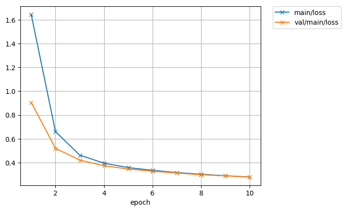
ロスの変遷のグラフが出力されますので見てみます。
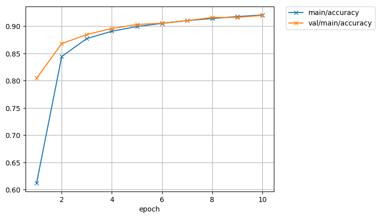
精度のグラフはこうなります。
なお、この程度の学習でしたらSurface Pro6(Core i5-8250U)でも数分で計算が終わります。
推論してみた
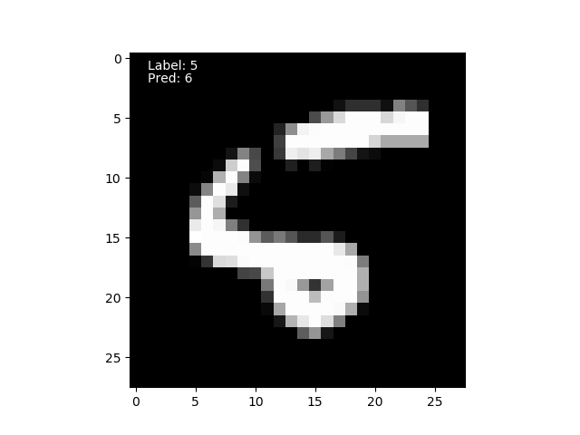
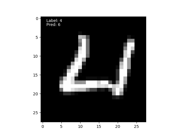
学習結果を使って、テスト用データから100枚の画像を推論してみました。
コードは前の投稿とほぼ同じです。推論にトレーナーは使いませんからね。学習データの読み込みのところが異なっています。
import pickle
import matplotlib.pyplot as plt
import numpy
from chainer.datasets import split_dataset_random
import chainer
import chainer.links as L
import chainer.functions as F
from chainer import serializers
# ネットワークの定義
class MLP(chainer.Chain):
def __init__(self, n_mid_units=100, n_out=10):
super(MLP, self).__init__()
# パラメータを持つ層
with self.init_scope():
self.l1 = L.Linear(None, n_mid_units)
self.l2 = L.Linear(n_mid_units, n_mid_units)
self.l3 = L.Linear(n_mid_units, n_out)
def __call__(self, x):
# データを受け取った際のforward計算
h1 = F.relu(self.l1(x))
h2 = F.relu(self.l2(h1))
return self.l3(h2)
# データセットの読み込み
with open('test.pickle', mode='rb') as fi1:
test = pickle.load(fi1)
# ネットワークのインスタンスを作る
infer_net = MLP()
# 学習データを読み込む
serializers.load_npz('mnist_result/snapshot_epoch-10', infer_net, path='updater/model:main/predictor/')
# テスト用のバッチデータを作る
test_batch_size = 100
t = [] # 画像のラベル
x, tt = test[0] # xが画像のデータ
t.append(tt)
for i in range(1,test_batch_size):
xt, tt = test[i]
t.append(tt)
x = numpy.vstack((x,xt))
# ネットワークと同じデバイス上にデータを送る
x = infer_net.xp.asarray(x)
# モデルのforward関数に渡す
with chainer.using_config('train', False), chainer.using_config('enable_backprop', False):
y = infer_net(x)
# Variable形式で出てくるので中身を取り出す
y = y.array
# 予測確率の最大値のインデックスを見る
pred_label = y.argmax(axis=1)
# 予測に失敗したデータの抽出
failed_index = []
for i in range(len(pred_label)):
if t[i] != pred_label[i]:
failed_index.append(i)
print('Failed: n = ', len(failed_index), ' / ', len(pred_label))
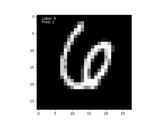
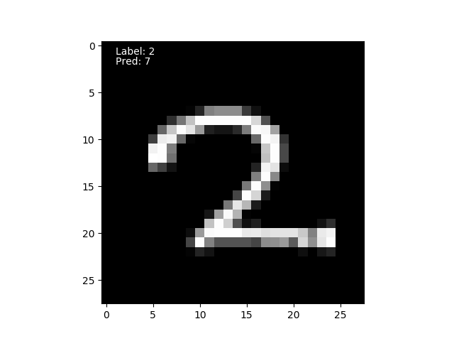
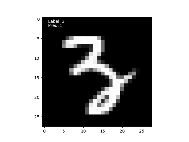
# 予測に失敗した画像の表示
for i in range(len(failed_index)):
label_text = 'Label: ' + str(t[failed_index[i]])
pred_text = 'Pred: ' + str(pred_label[failed_index[i]])
plt.imshow(x[failed_index[i]].reshape(28, 28), cmap='gray')
plt.text(1,1, label_text, color='white')
plt.text(1,2, pred_text, color='white')
plt.show()
やはり100枚中5枚が不正解でした。
公開日
広告
Chainerカテゴリの投稿
- ChainerCVで使える画像のデータ拡張
- ChainerCVで画像を出力する方法
- ChainerCVのResNetを使う
- ChainerCVのSSDに学習させてみた
- ChainerCVのデモンストレーションプログラムを読んでみた
- ChainerCVのデモンストレーションプログラムを読んでみた(推論編)
- Chainerが出力するネットワーク構造図をGraphvizで見る
- Chainerで数字を分類してみた
- ChainerのSSDのデモで物体検出をしてみる
- Chainerのチュートリアルを試してみた
- Chainerのチュートリアルを試してみた(ChainerCVでデータ拡張編)
- Chainerのチュートリアルを試してみた(データ拡張編)
- Chainerのチュートリアルを試してみた(トレーナー編)
- Chainerのチュートリアルを試してみた(畳み込みを深くする編)
- Chainerのチュートリアルを試してみた(畳み込み編)
- Chainerのデータセットの作り方(ラベル付き画像編)
- VoTTのPascal VOC出力をChainerCVのデータセットとして読み込んでみた